1.In Depth Insights

When the action of an operator on a function yields the original function multiplied by a constant, that function is called an eigenfunction. The constant factor ensuring this equality is known as the eigenvalue. More formally, if an operator $Â$acts on a function $f$such that:

$$Âf = af$$



then $f$ is an eigenfunction of $Â$, and $a$is the corresponding eigenvalue. Such an expression is termed an eigenvalue equation. The time-independent Schrödinger equation in quantum mechanics represents a prime example of an eigenvalue equation; other eigenvalue equations, such as those governing angular momentum, are likewise of central importance in quantum theory.



2. Mathematical Representation

Many fundamental problems across physics can be cast into the general form:

$$Aψ = λψ$$



where $A$is a linear operator acting on a Hilbert space, $ψ$is an element of that space (a state function), and $λ$is a scalar constant. While the operator $A$is known, both the eigenvalue $λ$and the function$ψ$are unknown. The central objective is to solve this equation, as its solutions correspond to functions $ψ$that remain invariant under the operation, up to an overall scaling factor $λ$. The German prefix Eigen translates loosely to "own", "peculiar", or "inherent". A function$ψ$satisfying this relation is an eigenfunction, and the associated scalar$λ$is its eigenvalue. The requirement that the operator A leaves $ψ$unchanged aside from scaling by$λ$imposes a severe restriction on the admissible forms of$ψ$. To appreciate the physical significance of these equations, consider the following examples:



1. Standing waves on a vibrating string: Resonant standing modes are those in which the restoring force acting on elements of the string (denoted by $Aψ$) is directly proportional to the displacement $ψ$from equilibrium.

2. Rigid-body rotation: The angular momentum L and angular velocity $ω$of a rigid body are three- dimensional vectors $(3-D)$related by:

$$L = Iω$$



where I denotes the 3×3 moment of inertia tensor. Here, $ω$defines the instantaneous axis of rotation, while $L$specifies the axis of angular momentum. The condition that these two axes coincide—which defines the principal axes of inertia—is given by$L = λω$, with $λ$being a proportionality constant. Substituting this into the constitutive relation yields:

$$Iω = λω$$



This represents an eigenvalue problem in which the operator is the matrix I, and the eigenfunction (conventionally termed an eigenvector) is $ω$. 3. Schrödinger equation: The time-independent Schrödinger equation in quantum mechanics is an eigenvalue problem where the operator $A$corresponds to the Hamiltonian $H$, $ψ$is the wave function, and $λ = E$represents the measurable energy eigenvalue associated with the state $ψ$. A powerful method for solving eigenvalue problems involves expressing them in terms of a complete orthonormal basis, . In this representation, the abstract operator $A$and the function $ψ$are mapped to a matrix $A$and a column vector$c$, whose elements are given by the inner products:

$$a_{ij}=\langle\phi_i|{A}|\phi_j\rangle,\qquad c_i=\langle\phi_i|\psi\rangle$$



Consequently, the original eigenvalue problem reduces to a matrix eigenvalue equation:

$$Ac = λc$$



The vectors$c$satisfying this system are referred to as eigenvectors. Once the matrix system is solved, the eigenfunctions of the continuous problem can be reconstructed via the basis expansion:

$$\psi=\sum_i c_i\phi_i$$



In some instances—such as the inertia tensor discussed above—the problem is intrinsically discrete and finite-dimensional. Under such circumstances, there is no need to project the problem onto an infinite-dimensional basis; the eigenvectors represent the physical solutions directly.

Equivalence of Operator and Matrix Formulations Because we are dealing with linear operators acting on elements of a Hilbert space, expanding both the operator and the wave function in terms of an orthonormal basis yields a matrix equation that is completely equivalent to the underlying continuous problem. A crucial implication of this equivalence is that any theorem concerning the spectral properties of eigenvectors or eigenvalues derived via a matrix expansion applies equally to the original operator formulation. Solving the matrix problem is thus equivalent to solving the physical problem itself.

An Illustrative Example Consider a frictionless particle executing two-dimensional motion$(2-D)$inside an elliptical potential well:





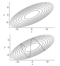
Figure 1:

Top: Contour plot of the potential well $V = x² - 5xy + 3y²$.

Bottom: Trajectory of a sliding unit-mass particle released from rest at $(-1.92, 8.0)$.



If the particle is released from rest at an arbitrary coordinate within the basin, it accelerates down the steepest descent along the negative gradient, which generally does not point toward the potential minimum at the origin. This misalignment produces a complex, non-periodic trajectory, as shown in the lower panel of Figure 1. The objective is to identify special trajectories along which the restoring force directs the particle straight toward the minimum, yielding uncoupled, one- dimensional simple harmonic motion.

To analyze this system analytically, consider a quadratic potential of the form:

$$V(x, y) = ax² + bxy + cy²$$



where the parameters$a, b$, and $c$are constrained such that the potential forms a convex elliptic basin with an isolated minimum at$x = 0, y = 0$. The Cartesian components of the conservative force acting at $(x, y)$are obtained via partial differentiation:

$$F_x=-\frac{\partial V}{\partial x}=-2ax-by, F_y=-\frac{\partial V}{\partial y}=-bx-2cy$$



For generic coordinates, $\frac{F_x}{F_y}\neq\frac{x}{y}$, confirming that the restoring force does not point along the position vector toward the origin at$x = y = 0$. For finding directions where the force points toward $x = y = 0$, writing these force equations in matrix form:

$$\begin{bmatrix} F_x\\ F_y \end{bmatrix} = \begin{bmatrix} -2a & -b\\ -b & -2c \end{bmatrix} \begin{bmatrix} x\\ y \end{bmatrix}$$



where $f, H,$and $r$are defined accordingly. The condition$\frac{F_x}{F_y}=\frac{x}{y}$is equivalent to requiring that $f$and$r$are proportional, which yields the eigenvalue problem:

$$Hr = λr$$



Here, $H$is known, while the eigenvalues $λ$and eigenvectors$r$ are to be determined. Rewriting this as a homogeneous linear system:

$$(H - λI)r = 0$$



Non-trivial solutions exist if and only if$r ≠ 0$, unless det$(H - λI) = 0$. Since $λ$is at our disposal, we seek values of $λ$such that:

$$\det(H-\lambda I)= \begin{vmatrix} h_{11}-\lambda & h_{12}\\ h_{21} & h_{22}-\lambda \end{vmatrix} =0$$



Evaluating the determinant produces the characteristic equation:

$$(h_{11}-\lambda)(h_{22}-\lambda)-h_{12}h_{21}=0$$



Solving this quadratic equation yields the eigenvalues$λ$. Substituting each root back into the homogeneous system det$(H - λI)$ allows solving for the vector $r$. This process can be repeated for all roots $λ$, providing the complete set of eigenvalues and eigenvectors.



3. Fundamental Properties



• Linearity: If$f(x)$ and $g(x)$ are eigenfunctions of a linear operator $L$ sharing the same eigenvalue, any linear combination$a·f(x) + b·g(x)$ is likewise an eigenfunction of $L$ with the same eigenvalue, where a and b are arbitrary scalars.



• Orthogonality: Under specific conditions, eigenfunctions corresponding to distinct eigenvalues are mutually orthogonal with respect to the inner product defined on the function space.



• Completeness: For many physically relevant problems, the set of eigenfunctions constitutes a complete basis for the state space, meaning that any function in that space can be expanded as a discrete series or continuous integral over these eigenfunctions.



• Normalization: Eigenfunctions can typically be normalized to unit norm. In quantum mechanics, this property is essential because eigenfunctions represent probability amplitudes.

When the characteristic equation det(H - λI) = 0 possesses repeated roots, the eigenvalue problem is said to be degenerate.



4. Applications

Eigenfunctions play a foundational role across multiple physical and engineering disciplines:



• Quantum Mechanics: The eigenfunctions of the Hamiltonian operator characterize the stationary states of quantum systems, and their eigenvalues determine observable quantities such as energy:

$$HΨ = EΨ$$



• Vibrational and Acoustic Analysis: Eigenfunctions describe the normal modes in oscillating systems such as taut strings, membranes, and elastic media.



• Signal Processing: In linear systems, eigenfunctions are used to analyze and design filters and solve differential equations modeling physical systems.



• Partial Differential Equations (PDEs): Eigenfunction expansions under separation of variables form the standard method for solving boundary value problems in mathematical physics and engineering.





5. Historical Context

The concept of eigenfunctions originated in eighteenth-century investigations of vibrating strings and trigonometric series expansions. Leonhard Euler and Daniel Bernoulli first explored the idea of using functions that are today recognized as eigenfunctions in characterizing oscillatory systems. In the early nineteenth century, Joseph Fourier achieved a major milestone by introducing Fourier series expansions. Subsequently, Charles-François Sturm and Joseph Liouville established the mathematical foundation of eigenvalue problems through Sturm–Liouville theory in the 1830s and 1840s. Their framework was later generalized by Lord Rayleigh and Edmund Titchmarsh, solidifying eigenfunction analysis as a cornerstone of modern mathematical physics and the solution of partial differential equations.



6. References

1. Mortimer, R. G., & Blinder, S. M. (2023). Mathematics for Physical Chemistry. Elsevier.

2. Arfken, G. B., Weber, H. J., & Harris, F. E. (2011). Mathematical Methods for Physicists: A Comprehensive Guide. Academic Press.

3. DeepAI Glossary: Eigenfunction. Retrieved from: https://deepai.org/machine-learning-glossary- and-terms/eigenfunction