1. In Depth Insights
Suppose a particle of mass moves along the axis under the influence of a specified force . The central objective of classical mechanics is to determine the position of the particle at any arbitrary time. Once velocity is obtained, dynamical variables such as momentum and kinetic energy can be directly calculated. To find the trajectory , we employ Newton's second law, which yields when supplied with appropriate initial boundary conditions such as and velocity at .
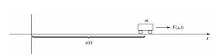
Figure: A particle constrained to motion in one dimension under the action of a specified force.
The approach of quantum mechanics differs fundamentally from this classical paradigm. In quantum mechanics, rather than seeking the particle's deterministic trajectory, we seek the wave function , obtained by solving the time dependent Schrödinger equation:
Planck's reduced constant in this differential equation is defined as:
The Schrödinger equation plays a role analogous to Newton's second law: given suitable initial conditions such as the wave function at, the equation uniquely determines for all future times, precisely as Newton's second law determines in classical mechanics.
What physical entity does the wave function represent, and what operations can be performed with it? A point particle is localized in space, whereas a wave function is distributed across space, being a function of spatial coordinates at each instant of time . How can such an extended spatial entity describe the state of a localized particle? The resolution was provided by Born's statistical interpretation, which states that the squared absolute magnitude of the wave function yields the probability density of locating the particle at position at time . More precisely, the probability of finding the particle within the spatial interval between points and at time is given by the integral:
Geometrically, this probability equals the area under the curve of between points and . For the wave function profile shown below, the probability of finding the particle near point, where is large, is considerably higher than the probability of finding it near point .
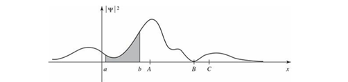
Figure: A standard wave function profile. The shaded area represents the probability of finding the particle between coordinates and . The particle is significantly more likely to be found near point than near point .
This statistical interpretation introduces intrinsic indeterminism into quantum mechanics. Even when everything knowable about a state is known through the complete wave function, one cannot predict with certainty the exact outcome of a single position measurement. Quantum mechanics instead provides statistical information regarding the probability distribution of possible outcomes.
2. Key Principles
1. Normalization
The wave function must be square integrable to ensure that the total probability of locating the particle somewhere across all space equals unity. Mathematically, this condition requires:
In three dimensional space, the normalization integral evaluates across the volume element :
2. Statistical Interpretation
The modulus squared of the wave function represents the spatial probability density for locating the particle at a specified coordinate and time.
3. Linearity and Superposition
The Schrödinger equation is a linear differential equation, meaning that if and are valid solutions, any arbitrary linear superposition of these solutions is likewise a valid solution.
4. Continuity
The wave function must remain continuous throughout space. Because spatial derivatives appear within the Schrödinger equation, the first derivative of the wave function must also be continuous across physical boundaries where potentials remain finite.
5. Complex Character
The wave function is inherently a complex valued function comprising both real and imaginary components. Observable physical quantities derived from it, including spatial probability distributions, evaluate strictly to real numbers.
6. Wave Function Collapse
Conducting a measurement forces the wave function to collapse into an eigenstate associated with the measured observable. Prior to measurement, the physical system occupies a coherent linear superposition of states; upon observation, the state vector projects abruptly onto a single eigenstate.
7. Dynamical Evolution
The temporal development of the state is governed by the time dependent Schrödinger equation. For a nonrelativistic quantum system, this dynamics takes the form:
where represents the Hamiltonian operator corresponding to the total energy of the physical system.
8. Boundary Conditions
Physical wave functions must satisfy specific boundary constraints, such as vanishing smoothly as spatial coordinates approach positive or negative infinity, ensuring normalizability and physical admissibility.
9. Orthogonality
Eigenstates associated with distinct quantum eigenvalues, such as distinct energy levels, are mutually orthogonal. Their inner product integral over all space evaluates strictly to zero when :
3. Applications
The wave function is the primary descriptive instrument across theoretical and applied quantum physics. Essential applications include:
- Quantum State Description: Provides complete quantum state information, enabling the extraction of expectation values for position, momentum, and energy.
- Probability Density Evaluation: Yields exact probability densities for locating a particle across space.
- Quantum Tunneling: Describes the finite probability of particles penetrating energetic potential barriers that are classically forbidden.
- Interference and Coherence: Accounts for constructive and destructive quantum interference across beam splitters and multi path interferometers.
- Energy Quantization: Solving the stationary Schrödinger equation with physical boundary conditions yields discrete energy eigenvalues and bound states.
- Measurement Predictions: Determines the complete statistical distribution of measurement outcomes for physical observables.
- Quantum Computing: Formalizes state vectors and multi qubit register dynamics within quantum processors.
- Quantum Field Theory: Generalizes wave functional formulations to evaluate relativistic probability amplitudes of field configurations.
- Harmonic Oscillator: Supplies quantized stationary state profiles for vibrational modes across molecular and solid state physics.
4. Historical Milestones
1. Louis de Broglie and Matter Waves (1924)
The conceptual origin of the wave function traces back to Louis de Broglie's 1924 hypothesis proposing that material particles exhibit wave characteristics analogous to radiation photons. De Broglie formulated the fundamental relation linking wavelength to momentum :
This relation supplied the theoretical foundation for associating an undulating mathematical entity, the wave function ψ(x, t), with material particles.
2. Erwin Schrödinger and the Wave Equation (1926)
In 1926, Erwin Schrödinger formulated wave mechanics, establishing a differential wave equation governing the continuous spatial and temporal evolution of matter waves. Schrödinger demonstrated that physical states can be represented by , whose dynamics are governed by:
where is the Hamiltonian operator and is Planck's reduced constant.
3. Max Born's Statistical Interpretation (1926)
Shortly after Schrödinger published his wave mechanics, Max Born proposed the probabilistic interpretation of the wave function. Born clarified that is not a classical physical fluid dispersed in space, but rather a probability amplitude whose squared magnitude yields the probability density of finding the particle at a specific location. This departure from deterministic classical mechanics established one of the foundational axioms of quantum mechanics.
4. Schrödinger's Conceptual Shift
Although Schrödinger originally regarded the wave field as a physical charge density distribution, he subsequently accepted that the function acts as a mathematical apparatus yielding statistical outcomes. Nevertheless, he remained deeply skeptical of state reduction postulates and the Copenhagen interpretation.
5. Copenhagen Interpretation (1927)
Formulated primarily by Niels Bohr and Werner Heisenberg during the late 1920s, the Copenhagen interpretation formalized the intrinsic indeterminism of quantum states. According to this view, the wave function contains all knowable physical information, while the measurement process induces a nonunitary collapse into an eigenstate of the measured observable.
5. References
Griffiths, D. J. (2018). Introduction to Quantum Mechanics (3rd ed.). Pearson.
Feynman, R. P., Leighton, R. B., & Sands, M. (1965). The Feynman Lectures on Physics. Addison Wesley.
Shankar, R. (2011). Principles of Quantum Mechanics. Springer.
Peskin, M. E., & Schroeder, D. V. (1995). An Introduction to Quantum Field Theory. Westview Press.
Cohen Tannoudji, C., Diu, B., & Laloë, F. (1977). Quantum Mechanics. Wiley.